


Credit: Image by Arbron on Flickr. Some rights reserved
To some reporters, data journalism might sound daunting – but it needn't be.
Just a handful of basic spreadsheet methods can help you start finding stories in data, whether that is crime stats, hospital admittance figures, property prices or school results.
Financial Times data journalist John Burn-Murdoch will be going 'beyond the basics' with a session on spreadsheet skills at the news:rewired digital journalism conference in London this Wednesday (23 July).
In the session, he will explain how to find news lines in large, cluttered datasets, and how to join two datasets with common features.
Until then, however, here are five everyday spreadsheet functions that will help you get started in data journalism.
The following functions apply to Microsoft Excel but similar features exist in all spreadsheet packages, including online services such as Google Drive.
As a general rule, if you are not comfortable typing in formulas manually, your best friend is the Formula Wizard button 'fx' which is to the left of the formula field, above all your data.
And even if you find yourself clicking the wrong cells, hitting 'escape' or clicking the 'cross' button will allow you to start over.
1. Adding
Figures displayed across any number of rows and columns can be easily added together using the SUM feature.
To do this, first click on an empty cell where you want the result to be displayed, and in this cell, type = SUM(
Next, highlight the area containing the figures to be added (from the first to the last cell containing data).
This will add the list of cells you have highlighted into your formula. Close the brackets ) and press enter.
For example, if you have 10 figures in cells in column 'B', your formula might now read =SUM(B2:B11)
This formula can be copied and pasted into other columns to add these up without having to retype the formula.
If you are adding all the figures across, say, 10 rows and four columns, your formula might read something like =SUM(B2:E11)
You can also add up numbers from some columns but not others by inserting a comma after highlighting each column, eg: =SUM(A2:A11,C2:C11,E2:E11)
You can also add individual cells without using SUM. To do this, type = then click your first cell, then type + and do this for each cell in turn, pressing + inbetween each click. This might, for example, create a formula like =A1+B7+C4+D9
Press enter when you have added the last cell you wish to add up, and the total will appear.
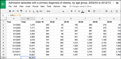
Screengrab from Google Drive using sample data from data.gov.uk
2. Averaging
There are different types of 'average' but perhaps the most commonly used is 'mean'. This is where you add up all the figures and divide the result by how many of them there are. Excel has an 'average' function that will calculate this for you.
To do this, pick an empty cell where the final calculation will appear.
Type =AVERAGE( and then highlight all the cells containing data that you want to find the average of.
Close the brackets, typing ), and hit enter.
The same principles apply as above with adding – for example: multiple columns could be combined with =AVERAGE(B2:E11) or alternate columns (AVERAGE=B2:B11,D2:D11,F2:11)
There are two other types of average: MODE( ) – which works out which number appears the most times – and MEDIAN( ) which works out which number would be in the middle if all the numbers were lined up in ascending order.
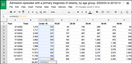
Screengrab from Google Drive using sample data from data.gov.uk
3. Sorting
Excel can automatically sort cells (or rows) in columns for you, alphabetically or numerically.
To do this, first highlight the cells you want to sort.
If these are in a single column that needs to be sorted simply in ascending numerical (or alphabetical) order, press the A->Z button in the toolbar. To reverse the order, use the Z->A button.
More complex sort functions are available for cells across multiple columns by using the 'sort' button next to these in the toolbar.
First, highlight all of your data, then click 'sort' and a pop-up window will appear, giving you the choice of which column to sort by. You can sort by multiple columns, telling Excel to first sort by information in column A, then by information in column G, for example, if you want to arrange information in multiple ways.
In the 'order' dropdown list, select the order that you want to apply to the sort operation — alphabetically or numerically, ascending or descending.
It is important that all of your data is selected, otherwise Excel will sort one column but leave the rest untouched, meaning the data might no longer line up or make sense.
4. Filtering
If your worksheet contains a lot of data, it can be difficult to find information quickly. Filters can be used to narrow down the data, allowing you to view only the information you need.
For example, you might have property prices for a whole town but only be interested in a particular road or neighbourhood.
Your data needs to include a header row, ideally with titles explaining what each column is about. (If it does not have a header row to start with, make one before starting this exercise.)
Start by selecting all the data. Then, click 'filter' (on the 'data' section of the menu ribbon). This will add small arrows by each of the column headings.
Click on the arrow on the column you wish to filter (if your sample data has a column for road names, or neighbourhoods, for example, that might be a useful one to use for filtering).
A window will appear with all the rows in that column and check boxes. Make sure only the data you wish to see is ticked, and you will see the information you do not need disappear. (Ticking a box again will bring the relevant row back, if you later decide you need it after all.)
Filtering is a way of temporarily hiding any content that doesn't match the criteria – and multiple filters can be applied.
To remove all filters, click the 'filter' command again. The dropdown arrows by the headings will disappear, and your hidden rows will reappear.
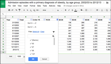
Screengrab from Google Drive using sample data from data.gov.uk
5. The paste special function
'Paste special' helps you link to data from other parts of your spreadsheet, for example another tab/sheet.
Select the cell or cells that contain the items or attributes you want to copy, and click 'copy'.
Click over to the part of your spreadsheet where the data should be pasted, click on the first available empty cell (top-left) and go to Edit>Paste Special.
For example, if you have copied the contents of a cell from Sheet1 of your project to Sheet2, the formula in Sheet2 might now read =$Sheet1.$B$1 (this being the reference to where the original data can be found).
John Burn-Murdoch, data journalist at the Financial Times, will be leading a session in spreadsheet skills for journalists at news:rewired on 23 July. Tickets have now sold out, but you can still buy a digital ticket which will allow you access to videos from the 10 main sessions at the event. For more details see the news:rewired website.
Free daily newsletter
If you like our news and feature articles, you can sign up to receive our free daily (Mon-Fri) email newsletter (mobile friendly).
Related articles
- Journalism and media events in 2024
- What can generative AI actually do for ordinary journalists?
- 'Journalism is extraordinarily resilient in the face of pressure and change'
- Workplace wellbeing interventions: what works, what doesn't and why?
- The Journalism Trust Initiative is rewarding transparent and trustworthy news


